Equations in research paper figures

You are writing a paper — a thesis, an arXiv preprint, an IEEE journal submission, a workshop note — and the figure you need has both a diagram and a typeset equation. A common workflow is to combine two or three tools: a diagramming app for the figure, a LaTeX renderer for the equation, and a final composition step. It works well, and many great figures are produced this way; the trade-off is that the equation is no longer editable from the same file, so revisions like “fix that one subscript” need a second pass through the renderer.

drawtonomy is one option that puts both on the same canvas. The diagram and the equation live in the same vector file, and the equation stays as editable LaTeX source until you decide otherwise.

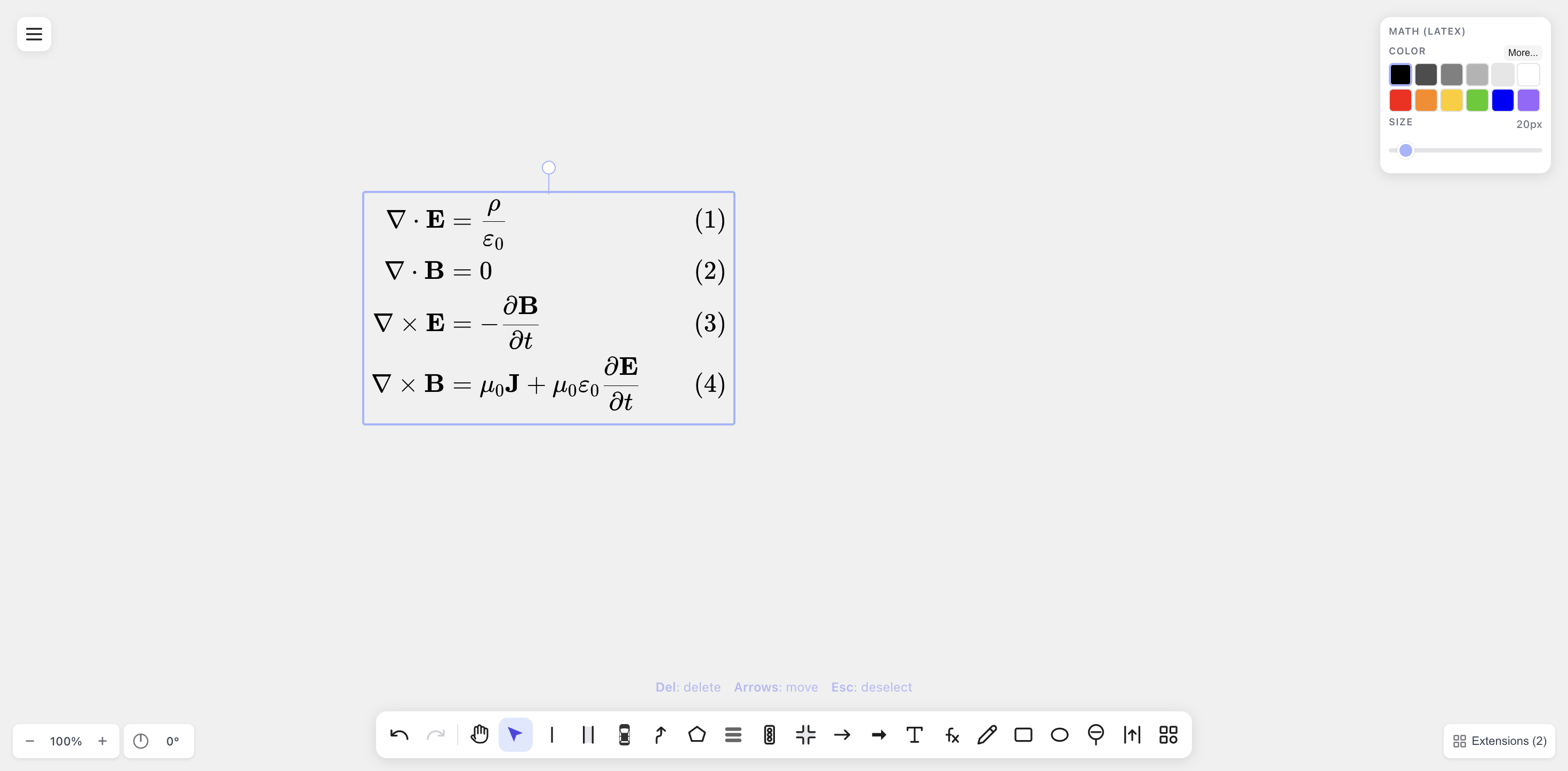
A typeset equation system (Maxwell’s equations) rendered with KaTeX on the drawtonomy canvas. The block is a single editable shape — double-click to bring the LaTeX source back.

Where drawtonomy fits among the alternatives

Each of these tools is excellent at what it’s designed for — drawtonomy is just shaped for a slightly different combination of constraints (one canvas, both diagram and equation editable).

• PowerPoint / Keynote are the universal choice for slides and many quick figures. They include their own equation editors, which are convenient, though they don’t keep LaTeX as a source format you can edit later.
• Inkscape / Illustrator give you superb vector control, and many papers’ final figures are polished there. When the equation comes from a separate LaTeX render, the LaTeX source lives in another file you maintain alongside the figure.
• Excalidraw / tldraw / Miro are excellent collaborative whiteboards. They focus on diagramming rather than typesetting, so equations are typically pasted in as images from a separate renderer.
• TikZ / pgfplots are the gold standard for fully programmatic, LaTeX-native figures, especially when precision matters. The trade-off is the iteration loop — each tweak goes through a compile.

drawtonomy sits between a slide tool and TikZ: a 2D vector canvas with a built-in KaTeX renderer that keeps your LaTeX source. If your figure naturally splits diagram and equation across separate tools, the existing toolchain is fine; drawtonomy is most useful when you want both in one editable file.

A practical workflow

1. Sketch the diagram on the canvas. Lanes / vehicles / pedestrians for an autonomous-driving paper. Rectangles + arrows for a controls block diagram. Polygons + path arrows for a method overview. Any combination of drawtonomy’s shapes is fair game — the Math shape is one of them.

2. Add the equation with the Math (fx) tool. The KaTeX preview renders live. Use \begin{align} for multi-line systems; KaTeX handles the equation numbering for you.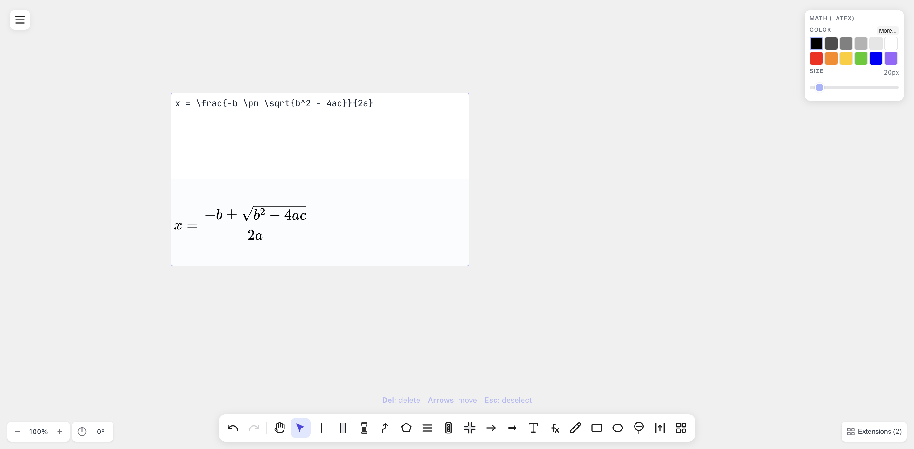

   

   Live KaTeX preview while typing the quadratic formula — top half is LaTeX source, bottom half is the rendered output.

3. Style for print. Most journals still print in grayscale. Pick black or dark-grey for equations; match the size to the diagram’s body text. The size slider goes up to 200 px for poster figures.

   

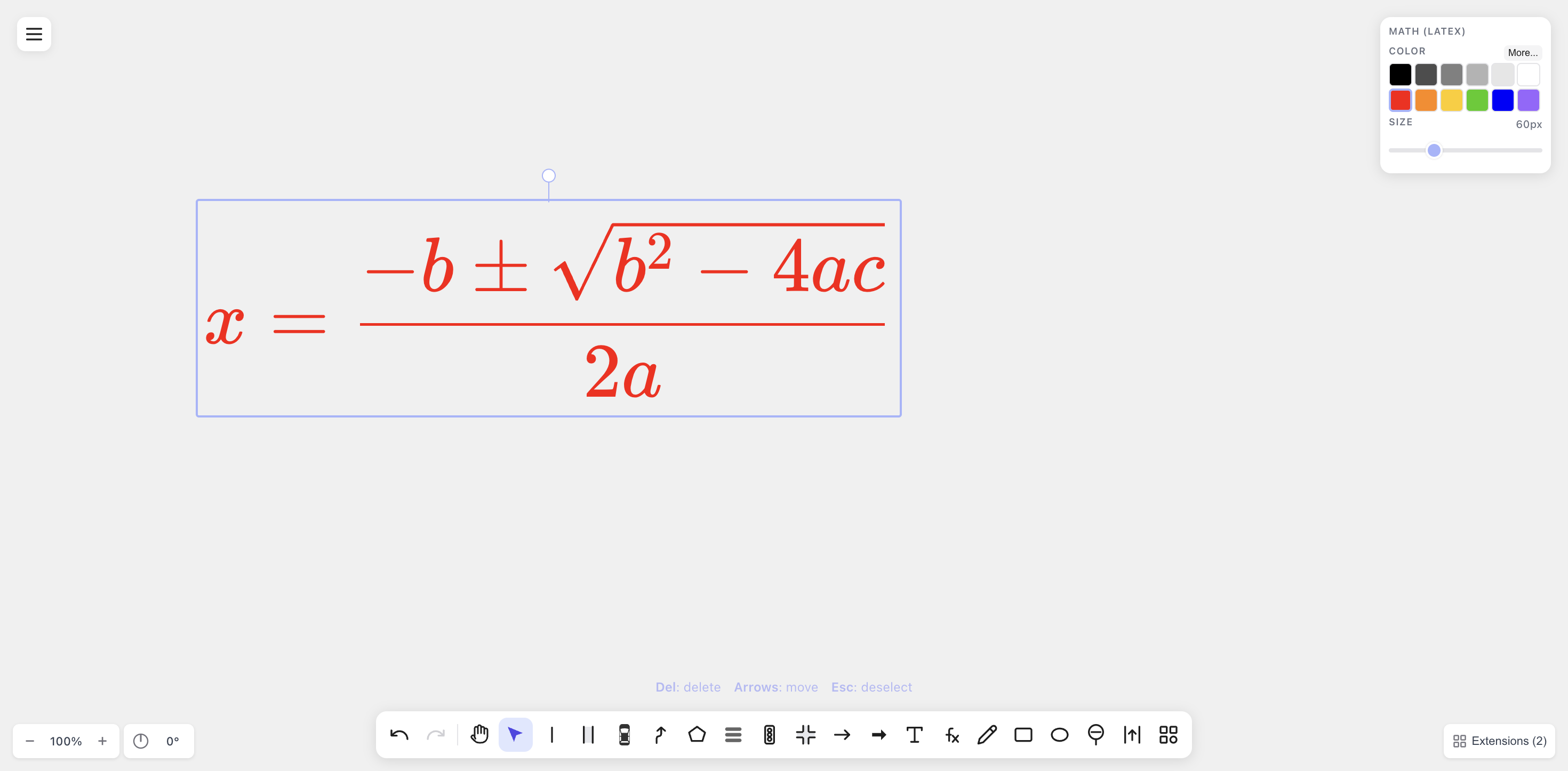
   Color and size are exposed in the Math (LaTeX) panel — pick a paper-safe black for grayscale prints, or a larger size for poster figures.

4. Export PDF for LaTeX builds. All glyphs (including the \sqrt vinculum) are converted to vector paths via opentype.js, so the file is self-contained — no font dependency, no pdflatex complaints. \includegraphics{...} drops it straight into your figure.

5. Save .drawtonomy.svg as the source of truth. When a reviewer asks for a variant (“can you replace \sigma with \rho?”), you reopen the .drawtonomy.svg in drawtonomy, double-click the equation to edit the LaTeX, re-export PDF. No redrawing.

LaTeX integration tips

• \includegraphics{equation.pdf} is the most reliable path for a paper. drawtonomy’s PDF export is path-based, so it works with any LaTeX engine (pdflatex, xelatex, lualatex).
• SVG + the svg package also works but depends on Inkscape on the build machine. Predictable for local builds, finicky on CI. Convert to PDF locally and check the PDF in.
• EPS is available for older latex + dvips toolchains; same path-based fidelity as the PDF.
• Fonts. Because text is path-converted, you don’t need to match the paper’s body font. The equation will look like KaTeX (Computer-Modern-style) regardless of the document’s font choice — which is usually what you want anyway.

Beyond autonomous driving

This use case is filed under autonomous-driving docs because drawtonomy started as a driving-scenario tool, but the Math shape is generic. The same workflow works for:

• Machine-learning method figures (loss equations next to the network diagram).
• Controls papers (transfer-function blocks with the LaTeX form beside each block).
• Signal-processing figures (Fourier-pair illustrations).
• Physics or chemistry papers (with \ce{} for reactions).
• Mathematics papers (proof figures with theorem statements typeset alongside).

If you can put it on a whiteboard, drawtonomy can hold it.

When this isn’t the right tool

• Equations that live inside a paragraph of text. Those belong in your LaTeX source, not in a figure.
• Dynamic plots driven by data — keep using matplotlib / pgfplots / TikZ for graphs.

See also

• Tutorial: Your first equation
• Guide: Add LaTeX equations
• Use case: figures for autonomous driving papers
• Reference: Math shape