Equations next to autonomous-driving figures
This is the cross-over use case for drawtonomy’s two strongest features at once: the autonomous-driving shapes (lanes, vehicles, paths, intersections) and the Math (KaTeX) shape.
It comes up surprisingly often in self-driving research papers. You don’t just want a picture of the scenario. You want the picture and the equation that describes the model — the cost function, the controller, the kinematic update — so the reader can map symbols back to the world.
A KaTeX-rendered formula sits as a normal shape on the canvas — drop it next to lanes, vehicles, and trajectories to build a single self-contained figure.
When this matters
Section titled “When this matters”- Trajectory prediction. Show three predicted future paths for the ego vehicle, with the model’s loss function typeset next to them.
- Motion planning. Show a candidate trajectory in the lane
scene, with the planning objective
\min \sum_t \| x_t - x_t^{ref} \|^2 + \lambda u_t^2rendered alongside. - Control. Show a vehicle following a curve, with the feedback controller’s equation next to the relevant geometry.
- Perception evaluation. Show a lane / pedestrian scene with the IoU or AP metric formula displayed next to it.
- Behaviour models. A pedestrian-crossing scene with the social-force / IDM equation rendered next to the agent.
In each case, the equation is part of the figure, not a caption.
The drawtonomy workflow
Section titled “The drawtonomy workflow”-
Draw the scene first. Lanes with the Lane Tool, vehicles from the Vehicle templates, trajectories with the Path tool — exactly as in the Your first three lanes tutorial.
-
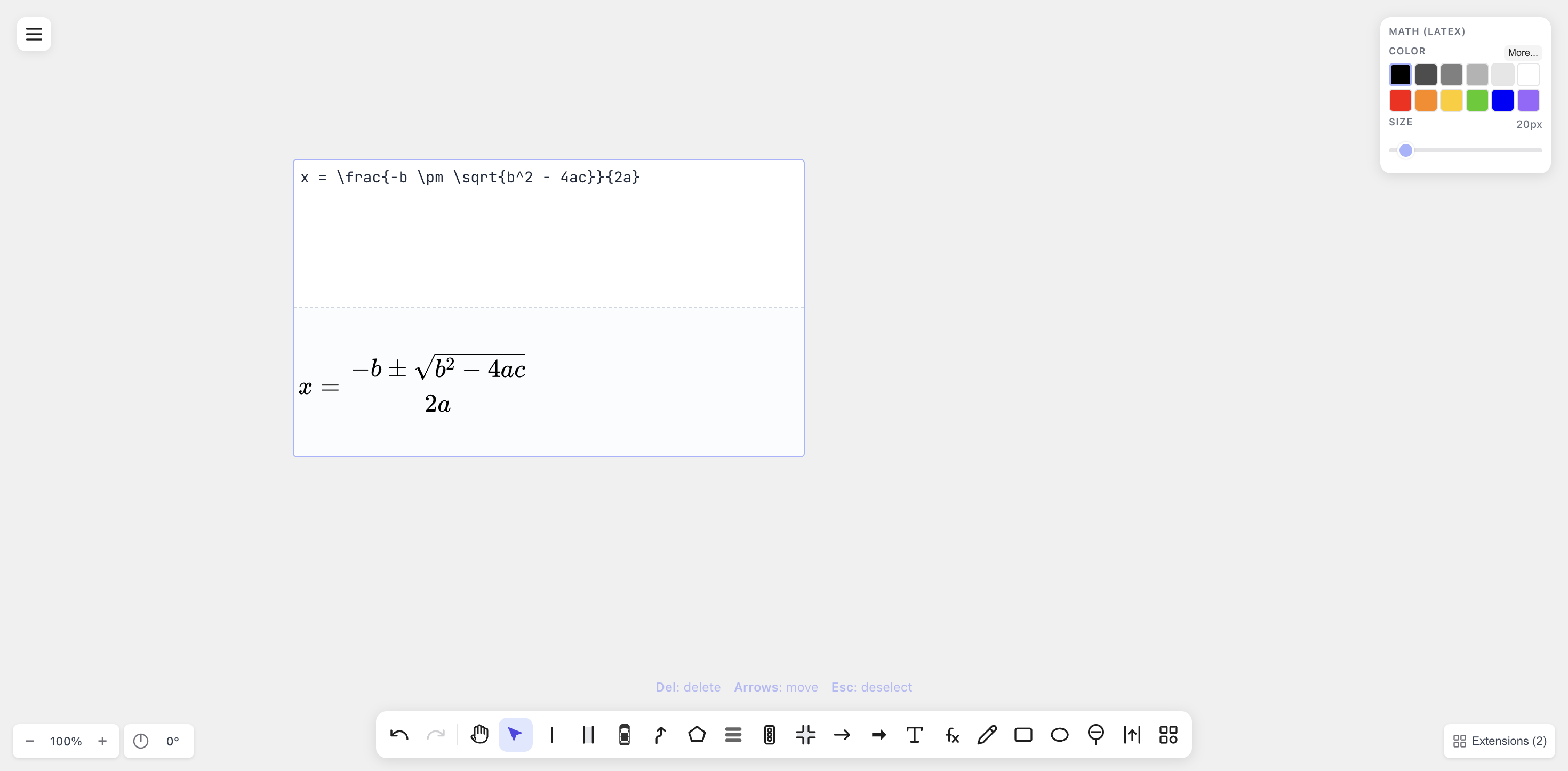
Place the equation with the Math (
fx) tool. Put it where it’ll read clearly — usually above or below the scene, or to one side.
The Math tool sits next to the Text tool in the bottom toolbar —
/is the keyboard shortcut. -
Tie symbols to the scene. Use LineArrows or Text shapes to connect, say, the
x_tin the equation to the relevant vehicle on the canvas. drawtonomy’s Snap feature helps the arrow latch to either side. -
Export PDF.
\includegraphics{...}it into your paper. The math glyphs and lane/vehicle paths are all vectors in the same file.
Practical tips
Section titled “Practical tips”- Match the equation size to the scene size. A 20 px equation next to a 600 px lane diagram disappears. Bump the size slider to 32 – 48 px to read well at journal-figure scale.
- Keep a
.drawtonomy.svgsource. When a reviewer asks to replace\sigmawith\rho, double-click the equation and retype — the lanes and vehicles don’t move. - Equation numbering vs. caption numbering. If your figure
has multiple equations and you want them numbered, use
\begin{align}so the numbers(1)(2)(3)are part of the rendered SVG. Otherwise the paper’s\label{}system has no way to reference equations inside a figure. - Colour for emphasis. Recolouring the relevant term of the equation requires using two adjacent Math shapes (one black, one red) — drawtonomy renders one equation as a single shape, so per-token colour isn’t supported.